ICML 2026

RL4RLA: Teaching ML to Discover
Randomized Linear Algebra Algorithms
Through Curriculum Design & Graph-Based Search

An RL framework that automatically discovers interpretable, symbolic RLA algorithms from first principles—no pretrained priors, no black-box outputs.

1 Pratt School of Engineering, Duke University 2 Department of Computer Science, Dartmouth College
*Equal contribution  ·  Corresponding: Yaoqing Yang
Code Paper arXiv BibTeX
Published at ICML 2026  ·  43rd International Conference on Machine Learning
4+
RLA paradigms rediscovered: Sketch-and-Precondition, Sketch-and-Project (Kaczmarz), Sketch-and-Solve, Newton Sketch; generalizes to eigenvalue problems
75–80%
End-to-end curriculum success rate across all linear-system targets
2–3×
Search cost reduction via Monte Carlo Graph Search over standard MCTS
100%
Newton Sketch discovery success — only full curriculum achieves it; all baselines fail

What is RL4RLA?

Randomized linear algebra (RLA) algorithms are a modern class of numerical linear algebra techniques that play an essential role in scientific computing and machine learning, with broad and growing adoption. However, their discovery remains mostly a manual process that requires deep expert knowledge and inspiration. While Reinforcement Learning (RL) offers a pathway to automation, standard approaches struggle with sparse reward landscapes and vast search spaces inherent to high-performing RLA algorithms.


In this paper, we present RL4RLA, a general RL framework that automates the discovery of interpretable, symbolic RLA algorithms. Unlike black-box approaches, our method builds explicit algorithms from basic linear algebra primitives, ensuring verifiable and implementable representations. To enable efficient discovery, we introduce:

  1. A numerical curriculum that progressively increments problem difficulty to encode inductive bias specific to the RLA domain.
  2. Monte Carlo Graph Search, which optimizes exploration by identifying and merging equivalent partial algorithms.

We demonstrate that RL4RLA rediscovers state-of-the-art methods, including sketch-and-precondition solvers, Randomized Kaczmarz, and Newton Sketch, and can be targeted to produce algorithms optimized for specific trade-offs between accuracy, speed, and stability. Code is available at github.com/Tim-Xiong/RL4RLA.

The RL4RLA Pipeline

RL4RLA frames algorithm discovery as building symbolic programs from linear-algebra primitives. Four components work together to make discovery tractable.
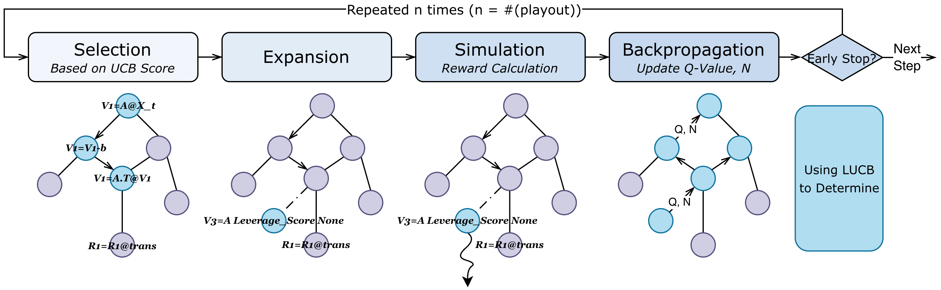
Overview of the RL4RLA framework
Figure 1: Overview of the RL4RLA framework, illustrated with the curriculum transition from Least Square Gradient Descent to Subsampled Least Square Gradient Descent. Top: At each curriculum stage, the search is initialized with a base algorithm and a problem environment (matrix properties, operator set, typed variables). The target algorithm is defined by augmenting the current algorithm. Bottom: Algorithm discovery is performed by Monte Carlo Graph Search. Each iteration selects actions via UCD, expands the partial algorithm by inserting operators, evaluates candidate algorithms through simulation reward computation, and backpropagates value estimates to update Q-values and visit counts. After each iteration, a LUCB-based criterion determines whether the current curriculum stage has been successfully completed.

Symbolic Algorithm Representation

Each candidate algorithm is an explicit symbolic program $\mathcal{A} = (\mathcal{P}_{\text{setup}}, \mathcal{P}_{\text{iteration}})$ built from typed linear-algebra primitives (SKETCH, HHQR, MATVEC, INV, …). Programs are directly executable and human-inspectable.

Curriculum-Guided Discovery

A sequence of staged refinements progressively increases problem difficulty. Each stage introduces exactly one failure mode (ill-conditioning, non-square, high-leverage) resolved by one new algorithmic component. Deep search becomes a chain of shallow problems.

Monte Carlo Graph Search

MCGS operates on a DAG rather than a tree, merging equivalent partial algorithms reached via different action orderings. This reduces growth from $O(b^d)$ tree nodes to $O(|\mathcal{S}|)$ unique states, achieving 2–3× search cost reduction.

Algorithm Tree

Starting from an empty program, RL4RLA navigates a DAG of increasingly sophisticated RLA algorithms. Hover over nodes to learn about each method.

Empty Landweber Iteration Least Square GD Preconditioned GD Gradient Descent Full Newton Method Block Rand. Kaczmarz Subsampled LS GD Subsampled Precond. GD Sketched Precond. GD Precond. Weighted SGD Newton Sketch Base Sketch & Precondition Sketch & Project Sketch & Solve Newton

Four RLA Paradigms

Sketch-and-Precondition

Constructs a cheap randomized preconditioner from a sketched version of $A$. Given $Ax=b$, a sketching operator $S \in \mathbb{R}^{s \times m}$ yields $SA = QR^{-1}$ such that $\kappa(AR) = \mathcal{O}(1)$, enabling fast preconditioned gradient updates. Recovers the core idea behind Blendenpik and LSRN.

// Setup (once)
R₁ ← Sketch(A)        // apply sketching matrix
R₁ ← QR(R₁ · A)      // compute QR of SA
R₁ ← Inv(R₁)          // invert R factor
R₁ ← R₁ · R₁ᵀ        // form preconditioner

// Iteration
v₁ ← MatVec(A, xₜ)   // Axₜ
v₁ ← v₁ − b
v₁ ← Aᵀ · v₁         // Aᵀ(Axₜ − b)
v₁ ← R₁ · v₁         // apply preconditioner
xₜ₊₁ ← xₜ − η · v₁
Recovers: Sketched Preconditioned Gradient Descent (Blendenpik)
Sketch-and-Project

Updates iterates by projecting onto randomly sketched subsystems. At each step, solves a small projected problem: $x_{t+1} = \arg\min_x \|x-x_t\|^2 \text{ s.t. } S_t Ax = S_t b$. Recovers Randomized Kaczmarz (single-row) and Block Randomized Kaczmarz (multi-row sketch).

// Iteration (no setup phase needed)
Sₜ ← Sample(rows of A, b)  // sketch matrix
r ← Sₜ·A·xₜ − Sₜ·b     // sketched residual
xₜ₊₁ ← xₜ − (SₜA)ᵀ · Inv((SₜA)(SₜA)ᵀ) · r

// Equivalent to projecting onto S_t Ax = S_t b
Recovers: Block Randomized Kaczmarz
Sketch-and-Solve

Directly solves a sketched least-squares problem: $\tilde{x} = \arg\min_x \|SAx - Sb\|^2$. Discovered on large overdetermined systems when edit distance is small, reducing complexity while preserving accuracy.

// One-shot solve
S ← Sketch(A, b)          // draw random sketch
 ← S · A                 // reduced system: s×n
b̂ ← S · b
x̃ ← LeastSquares(Â, b̂)   // solve sketched LS
Recovers: Subsampled Least Squares GD
Newton Sketch

Approximates the Hessian $H_t = A^\top D_t A$ via sketching: $\hat{H}_t = (SD_t^{1/2}A)^\top (SD_t^{1/2}A)$, reducing complexity from $O(mn^2)$ to $O(smn)$ while maintaining superlinear convergence. Applied to logistic regression. Only the full curriculum achieves 100% success; all partial curricula fail.

// Iteration (logistic regression)
Dₜ ← Diag(σ′(Axₜ))      // logistic weights
S ← Sketch(Dₜ^{1/2}·A)    // sketch weighted A
Ĥₜ ← Sᵀ · S               // approximate Hessian
gₜ ← Aᵀ · (σ(Axₜ) − y)  // gradient
xₜ₊₁ ← xₜ − Ĥₜ⁻¹ · gₜ    // Newton step
Recovers: Newton Sketch (Pilanci & Wainwright 2017)

Progressive Difficulty Staging

Deep algorithmic search is decomposed into shallow staged refinements. Each stage introduces one failure mode resolved by one new component. Click a stage to explore the progression.

Stage 0: Landweber Iteration Base
Problem Setup
$5 \times 5$, well-conditioned $(\kappa \approx 2)$
Failure Mode
None — base case
x_{t+1} = x_t − η (Ax_t − b)
✓ Fixed-point / Landweber iteration
Stage 1: Gradient Descent +AᵀA term
Problem Setup
$m \times n$ rectangular system
Failure Mode
Non-square system — need normal equations
x_{t+1} = x_t − η AT(Ax_t − b)
✓ Gradient Descent via normal equations
Stage 2: Preconditioned GD +Preconditioning
Problem Setup
$10000 \times 50$, ill-conditioned $(\kappa \gg 1)$
Failure Mode
Slow convergence due to high condition number
// Compute once: A = QR⁻¹
x_{t+1} = x_t − η RRTAT(Ax_t − b)
✓ Preconditioned GD (exact QR)
Stage 3: Sketched Preconditioned GD +Sketching
Problem Setup
Same, higher complexity penalty $w_{\text{comp}}$
Failure Mode
Full QR factorization too expensive
// Cheap sketch: SA = QR⁻¹
x_{t+1} = x_t − η RRTAT(Ax_t − b)
✓ Sketched Preconditioned GD ≈ Blendenpik
Stage 4: Uniform Row Subsampling +Stochasticity
Problem Setup
Same setup, uniform distribution
Failure Mode
Full-batch gradient inefficient per iteration
// Sₜ: uniform row sampling per iteration
x_{t+1} = x_t − η RRT(StA)T(StAx_t − Stb)
✓ Stochastic Preconditioned GD (uniform sampling)
Stage 5: Leverage-Score SGD +Importance Sampling
Problem Setup
Heavy-tailed $U$ in $A = U\Lambda V^\top$ (non-uniform leverage)
Failure Mode
Uniform sampling suboptimal for skewed leverage scores
// Sₜ: ℓ₂ row-norm (leverage-score) sampling
x_{t+1} = x_t − η RRT(StA)T(StAx_t − Stb)
✓ Preconditioned Weighted SGD (leverage-score sampling)
Key Insight: Decomposing the search for a 6-component algorithm into 5 shallow transitions transforms a globally sparse program space into a sequence of locally solvable refinements. Each stage introduces exactly one failure mode, keeping the reward landscape locally informative and the search horizon tractable. Once a correct base algorithm is provided, subsequent transitions become nearly deterministic (≥95–100% success).

Monte Carlo Graph Search

Standard MCTS treats the search space as a tree, causing exponential redundancy. MCGS merges equivalent states into a DAG, dramatically reducing search cost.

MCTS (Tree Search) Baseline
  • Tree grows $O(b^d)$ — exponential in depth
  • Equivalent partial programs re-explored as separate nodes
  • UCT assigns free bonuses to redundant nodes
  • Most compute wasted on re-generating seen programs
MCGS (Graph Search) Ours
  • DAG grows $O(|\mathcal{S}|)$ — only unique states
  • Equivalent states merged by exact program normalization
  • UCD action selection corrects for multi-parent nodes
  • Revisit rate 50–58%: majority of compute refines known states
  • 2–3× total search cost reduction across all curricula

Backpropagation updates (shared across all paths to merged state $s$)

$$N(s,a) \leftarrow N(s,a) + 1$$
$$\hat{Q}(s,a) \leftarrow \hat{Q}(s,a) + \frac{R - \hat{Q}(s,a)}{N(s,a)}$$

UCD action selection (corrects UCT's over-exploration on multi-parent nodes):

$$a' = \arg\max_{a \in \mathcal{A}(s)} \left[ \hat{Q}(s,a) + c \sqrt{\frac{\log N(s)}{N(s')}} \right]$$

(a) Unique-State Growth

Number of unique algorithmic states $|S|$ versus playout index. MCTS expands nearly linearly; MCGS saturates earlier, consistent with frequent transpositions and node merging.

(b) Revisit Rate

Revisit rate $1 - |S|/|V|$ versus playout index, where $|V|$ is total node visits. MCGS sustains a higher revisit rate throughout search, indicating greater reuse of shared states.

Search Efficiency Results

RL4RLA evaluated across five curricula. MCGS+UCD consistently achieves the lowest playout cost and best wall-clock time while maintaining competitive success rates.

Total Playouts to Complete Full Curriculum (lower is better)

Target Algorithm Method Total Playouts ↓ Time (s) ↓ Success Rate
Preconditioned Weighted SGD MCTS34,902380.7 75%
MCGS+UCT13,037193.2 80%
MCGS+UCD10,721191.1 80%
Block Randomized Kaczmarz
MCTS66,468468.0 75%
MCGS+UCT38,469307.8 80%
MCGS+UCD25,158205.0 75%
Subsampled Least Square GD
MCTS15,84710.4 75%
MCGS+UCT7,2308.3 80%
MCGS+UCD5,0618.9 80%
Sketched Preconditioned GD
MCTS17,655142.9 75%
MCGS+UCT8,03054.8 80%
MCGS+UCD6,03458.4 75%
Newton Sketch †
MCTS2,5575,949.6 100%
MCGS+UCT2,6825,265.4 100%
MCGS+UCD1,4164,480.9 100%

† Full four-stage curriculum required; all no-curriculum and partial-curriculum variants achieve 0% success. 20 runs per transition; LUCB early stopping.

Empirical CDF of Playouts-to-Success

As compositional depth increases, MCGS variants show pronounced advantages. On shallow targets all methods are comparable; on deep targets MCGS+UCD leads significantly.

(a) Landweber Iteration

Shallow target: all three methods discover the algorithm quickly, with MCGS variants having a slight edge.

(b) Sketched Preconditioned GD

Compositional target: MCGS variants show pronounced left shift; MCTS requires roughly 3× more playouts.

(c) Block Randomized Kaczmarz

Most compositional target: largest separation between methods. MCGS+UCD concentrates below 23k playouts; MCTS median exceeds 50k.

Beyond Least-Squares Problems

Domain adaptation requires only a thin interface layer. The core MCGS + curriculum logic transfers intact.

Interface additions for eigenvalue problems:

  • + One new primitive: VEC_NORMALIZE
  • + Rayleigh quotient-based reward: $\rho(x_t) = x_t^\top A x_t / \|x_t\|^2$
  • ± Same MCGS structure, same curriculum logic
Stage Size κ(A) Discovered SR
C0$n=5$$\approx 2$ Power Iteration 100%
C1$n=50$$\approx 10^2$ Power Iteration 100%
C2$n=500$$\approx 10^2$ Sketched Power Iter. 100%

5 seeds; MCGS+UCD. All three stages succeed.

Note: Chart below is for illustration only — data points are approximate reconstructions from the paper's figure. See the paper for exact results.

Eigenvalue Convergence (Rayleigh Quotient ρ → 1)

$\rho(x_t)$ over iterations; $\rho=1$ indicates exact recovery of $\lambda_{\max}$. C0/C1 rediscover power iteration; C2 (large $n$) rediscovers sketched power iteration.

Comparison with Program-Search Baselines

AlgoTune

Performs code-level optimizations (JIT, library swaps) on existing implementations. Produces dense deterministic solvers (Cholesky, LAPACK lstsq, L-BFGS) in all 5 variants. Does not compose new algorithmic structures.

FunSearch

Relies on pretrained LLM as mutation operator. Biases search toward training distribution. Scales poorly across diverse linear systems — higher runtime and noncompetitive residuals on both well-conditioned and ill-conditioned problems.

RL4RLA (Ours)

No pretrained priors. Searches explicitly over typed symbolic programs. Discovers interpretable RLA primitives: sketching, preconditioning, importance sampling — from scratch.

BibTeX

@inproceedings{xiong2026rl4rla,
  title     = {RL4RLA: Teaching ML to Discover Randomized Linear Algebra
             Algorithms Through Curriculum Design and Graph-Based Search},
  author    = {Xiong, Jinglong and Liu, Xiaotian and Wang, Ruoxin and
             Liu, Zihang and Zhou, Yefan and Yan, Yujun and Yang, Yaoqing},
  booktitle = {Proceedings of the 43rd International Conference on
             Machine Learning (ICML)},
  year      = {2026},
  eprint    = {2605.18004},
  archivePrefix = {arXiv},
  url       = {https://arxiv.org/abs/2605.18004},
}