Understanding Transformers from Scratch: A NumPy Implementation
Understanding Transformers from Scratch: A NumPy Implementation
In this blog post, we'll dive deep into the Transformer architecture by examining a pure NumPy implementation. The Transformer, introduced in the paper "Attention Is All You Need" by Vaswani et al., revolutionized natural language processing and has become the foundation for models like BERT, GPT, and T5.
By implementing a Transformer using only NumPy, we can understand the core concepts without the abstraction layers of deep learning frameworks. Let's explore each component of the architecture, the mathematics behind it, and how it's implemented in code.
Table of Contents
- The Transformer Architecture
- Layer Normalization
- Multi-Head Attention
- Positional Encoding
- Position-wise Feed-Forward Networks
- Encoder and Decoder Layers
- The Complete Transformer
- Conclusion
The Transformer Architecture
The Transformer architecture consists of an encoder and a decoder, each composed of multiple identical layers. Unlike recurrent neural networks (RNNs), Transformers process the entire sequence in parallel, using attention mechanisms to capture dependencies between tokens.
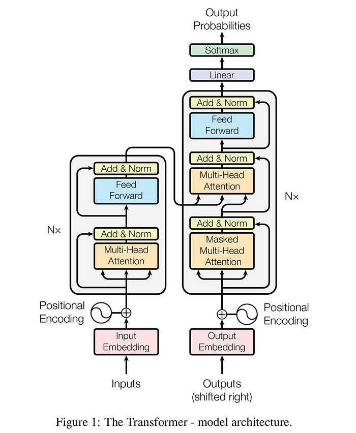
The key components of the Transformer are:
- Multi-Head Attention: Allows the model to focus on different parts of the input sequence
- Position-wise Feed-Forward Networks: Processes each position independently
- Layer Normalization: Stabilizes training by normalizing activations
- Positional Encoding: Adds information about token positions
- Residual Connections: Helps with gradient flow during training
Let's examine each component in detail.
Layer Normalization
Layer normalization normalizes the activations of the previous layer for each given example in a batch independently, rather than across a batch like batch normalization.
The Math
For an input vector $x$, layer normalization computes:
$$\text{LayerNorm}(x) = \gamma \cdot \frac{x - \mu}{\sqrt{\sigma^2 + \epsilon}} + \beta$$
Where:
- $\mu$ is the mean of the features
- $\sigma^2$ is the variance of the features
- $\gamma$ and $\beta$ are learnable parameters
- $\epsilon$ is a small constant for numerical stability
The Code
class LayerNorm:
    def __init__(self, dims, eps=1e-6):
        self.eps = eps
        self.gamma = np.ones(dims)
        self.beta = np.zeros(dims)

    def __call__(self, x):
        mu = np.mean(x, axis=-1, keepdims=True)
        var = np.var(x, axis=-1, keepdims=True)
        x_norm = (x - mu) / np.sqrt(var + self.eps)
        return self.gamma * x_norm + self.beta
The implementation follows the mathematical definition directly. We compute the mean and variance along the feature dimension, normalize the input, and then scale and shift using the learnable parameters gamma and beta.
Multi-Head Attention
Attention mechanisms allow the model to focus on relevant parts of the input sequence when producing an output. Multi-head attention runs multiple attention mechanisms in parallel, allowing the model to attend to information from different representation subspaces.
The Math
The scaled dot-product attention is defined as:
$$\text{Attention}(Q, K, V) = \text{softmax}\left(\frac{QK^T}{\sqrt{d_k}}\right)V$$
Where:
- $Q$ (query), $K$ (key), and $V$ (value) are matrices
- $d_k$ is the dimension of the keys
Multi-head attention is computed as:
$$\text{MultiHead}(Q, K, V) = \text{Concat}(\text{head}_1, \ldots, \text{head}_h)W^O$$
Where each head is:
$$\text{head}_i = \text{Attention}(QW_i^Q, KW_i^K, VW_i^V)$$
The Code
class MultiHeadAttention:
    def __init__(self, d_model, num_heads):
        self.d_model = d_model
        self.num_heads = num_heads
        self.d_k = d_model // num_heads
        self.W_q = np.random.randn(d_model, d_model) * 0.01
        self.W_k = np.random.randn(d_model, d_model) * 0.01
        self.W_v = np.random.randn(d_model, d_model) * 0.01
        self.W_o = np.random.randn(d_model, d_model) * 0.01

    def split_heads(self, x):
        batch_size = x.shape[0]
        x = x.reshape(batch_size, -1, self.num_heads, self.d_k)
        return x.transpose(0, 2, 1, 3)

    def scaled_dot_product_attention(self, Q, K, V, mask=None):
        scores = np.matmul(Q, K.transpose(0, 1, 3, 2)) / np.sqrt(self.d_k)

        if mask is not None:
            scores = np.where(mask == 0, -1e9, scores)

        attention_weights = np.exp(scores) / np.sum(np.exp(scores), axis=-1, keepdims=True)
        return np.matmul(attention_weights, V)

    def __call__(self, Q, K, V, mask=None):
        batch_size = Q.shape[0]

        Q = np.matmul(Q, self.W_q)
        K = np.matmul(K, self.W_k)
        V = np.matmul(V, self.W_v)

        Q = self.split_heads(Q)
        K = self.split_heads(K)
        V = self.split_heads(V)

        scaled_attention = self.scaled_dot_product_attention(Q, K, V, mask)

        scaled_attention = scaled_attention.transpose(0, 2, 1, 3)
        concat_attention = scaled_attention.reshape(batch_size, -1, self.d_model)
        output = np.matmul(concat_attention, self.W_o)

        return output
The implementation follows these steps:
- Project the input matrices using the weight matrices $W_q$, $W_k$, and $W_v$
- Split the projected matrices into multiple heads
- Compute scaled dot-product attention for each head
- Concatenate the attention outputs and project using $W_o$
The split_heads function reshapes the input to separate the heads dimension, and the scaled_dot_product_attention function implements the attention mechanism with optional masking.
Positional Encoding
Since the Transformer doesn't have recurrence or convolution, it needs positional encoding to make use of the order of the sequence. The original paper uses sine and cosine functions of different frequencies.
The Math
For position $pos$ and dimension $i$, the positional encoding is:
$$PE_{(pos, 2i)} = \sin\left(\frac{pos}{10000^{2i/d_{model}}}\right)$$ $$PE_{(pos, 2i+1)} = \cos\left(\frac{pos}{10000^{2i/d_{model}}}\right)$$
Where:
- $pos$ is the position in the sequence
- $i$ is the dimension index
- $d_{model}$ is the model's dimension
The Code
class PositionalEncoding:
    def __init__(self, d_model, max_seq_length=5000):
        pe = np.zeros((max_seq_length, d_model))
        position = np.arange(0, max_seq_length)[:, np.newaxis]
        div_term = 10000.0 **(np.arange(0, d_model, 2) / d_model)
        pe[:, 0::2] = np.sin(position / div_term)
        pe[:, 1::2] = np.cos(position / div_term)
        self.pe = pe[np.newaxis, :, :]

    def __call__(self, x):
        return x + self.pe[:, :x.shape[1], :]
The implementation creates a matrix of positional encodings for each position and dimension. Even dimensions use sine functions, and odd dimensions use cosine functions. The positional encoding is added to the input embeddings.
Position-wise Feed-Forward Networks
Each position in the sequence is processed by the same feed-forward network, which consists of two linear transformations with a ReLU activation in between.
The Math
The feed-forward network is defined as:
$$\text{FFN}(x) = \max(0, xW_1 + b_1)W_2 + b_2$$
Where:
- $W_1$, $W_2$, $b_1$, and $b_2$ are learnable parameters
- $\max(0, x)$ is the ReLU activation function
The Code
class PositionWiseFFN:
    def __init__(self, d_model, d_ff):
        self.W_1 = np.random.randn(d_model, d_ff) * 0.01
        self.W_2 = np.random.randn(d_ff, d_model) * 0.01
        self.b1 = np.zeros(d_ff)
        self.b2 = np.zeros(d_model)

    def __call__(self, x):
        Y1 = np.matmul(x, self.W_1) + self.b1
        Y1 = self.relu(Y1)
        Y2 = np.matmul(Y1, self.W_2) + self.b2
        return Y2

    @staticmethod
    def relu(x):
        return np.maximum(0, x)
The implementation follows the mathematical definition directly. It applies two linear transformations with a ReLU activation in between.
Encoder and Decoder Layers
The encoder and decoder layers combine the components we've discussed to process the input and output sequences.
Encoder Layer
Each encoder layer has two sub-layers:
- Multi-head self-attention
- Position-wise feed-forward network
Each sub-layer has a residual connection followed by layer normalization.
class EncoderLayer:
    def __init__(self, d_model, num_heads, d_ff, dropout_rate=0.1):
        self.mha = MultiHeadAttention(d_model, num_heads)
        self.ffn = PositionWiseFFN(d_model, d_ff)
        self.layernorm1 = LayerNorm(d_model)
        self.layernorm2 = LayerNorm(d_model)
        self.dropout_rate = dropout_rate

    def __call__(self, x, mask=None):
        attn_output = self.mha(x, x, x, mask)
        out1 = self.layernorm1(x + attn_output)  # residual connection
        ffn_output = self.ffn(out1)
        out2 = self.layernorm2(out1 + ffn_output)  # residual connection
        return out2
Decoder Layer
Each decoder layer has three sub-layers:
- Masked multi-head self-attention
- Multi-head attention over the encoder output
- Position-wise feed-forward network
Each sub-layer has a residual connection followed by layer normalization.
class DecoderLayer:
    def __init__(self, d_model, num_heads, d_ff, dropout_rate=0.1):
        self.mha1 = MultiHeadAttention(d_model, num_heads)
        self.mha2 = MultiHeadAttention(d_model, num_heads)
        self.ffn = PositionWiseFFN(d_model, d_ff)

        self.layernorm1 = LayerNorm(d_model)
        self.layernorm2 = LayerNorm(d_model)
        self.layernorm3 = LayerNorm(d_model)

        self.dropout_rate = dropout_rate

    def __call__(self, x, enc_output, look_ahead_mask=None, padding_mask=None):
        attn1 = self.mha1(x, x, x, look_ahead_mask)
        out1 = self.layernorm1(attn1 + x)  # residual connection

        attn2 = self.mha2(out1, enc_output, enc_output, padding_mask)
        out2 = self.layernorm2(attn2 + out1)  # residual connection

        ffn_output = self.ffn(out2)
        out3 = self.layernorm3(ffn_output + out2)  # residual connection

        return out3
The Complete Transformer
The complete Transformer combines the encoder and decoder layers, along with embedding layers and a final linear projection.
class Transformer:
    def __init__(
        self,
        num_layers,
        d_model,
        num_heads,
        d_ff,
        input_vocab_size,
        target_vocab_size,
        max_seq_length=5000,
        dropout_rate=0.1
    ):
        self.encoder_embedding = np.random.randn(input_vocab_size, d_model) * 0.01
        self.decoder_embedding = np.random.randn(target_vocab_size, d_model) * 0.01
        self.positional_encoding = PositionalEncoding(d_model, max_seq_length)

        self.encoder_layers = [
            EncoderLayer(d_model, num_heads, d_ff, dropout_rate)
            for _ in range(num_layers)
        ]

        self.decoder_layers = [
            DecoderLayer(d_model, num_heads, d_ff, dropout_rate)
            for _ in range(num_layers)
        ]

        self.final_layer = np.random.randn(d_model, target_vocab_size) * 0.01

    def encode(self, x, mask=None):
        x = np.matmul(x, self.encoder_embedding)
        x = self.positional_encoding(x)

        for layer in self.encoder_layers:
            x = layer(x, mask)

        return x

    def decode(self, x, enc_output, look_ahead_mask=None, padding_mask=None):
        x = np.matmul(x, self.decoder_embedding)
        x = self.positional_encoding(x)

        for layer in self.decoder_layers:
            x = layer(x, enc_output, look_ahead_mask, padding_mask)

        return x

    def __call__(self, inputs, targets=None):
        enc_output = self.encode(inputs)

        if targets is not None:
            dec_output = self.decode(targets, enc_output)
            final_output = np.matmul(dec_output, self.final_layer)
            return final_output

        return enc_output
The Transformer's forward pass consists of:
- Embedding the input and adding positional encoding
- Passing the embedded input through the encoder layers
- If targets are provided, embedding them and passing through the decoder layers
- Projecting the decoder output to the target vocabulary size
Conclusion
In this blog post, we've explored a pure NumPy implementation of the Transformer architecture. By breaking down each component and examining both the mathematics and the code, we've gained a deeper understanding of how Transformers work.
The key insights from this implementation are:
- Parallelization: Unlike RNNs, Transformers process the entire sequence in parallel, making them more efficient for training.
- Attention Mechanisms: The multi-head attention allows the model to focus on different parts of the input sequence.
- Positional Information: Since there's no recurrence, positional encoding is crucial for the model to understand sequence order.
- Residual Connections: These connections help with gradient flow during training.
This NumPy implementation serves as an educational tool to understand the inner workings of Transformers. For practical applications, you would typically use deep learning frameworks like PyTorch or TensorFlow, which provide optimized implementations and automatic differentiation.
By understanding the fundamentals of Transformers, you're better equipped to work with modern NLP models like BERT, GPT, and T5, which build upon this architecture.
References
- Vaswani, A., Shazeer, N., Parmar, N., Uszkoreit, J., Jones, L., Gomez, A. N., ... & Polosukhin, I. (2017). Attention is all you need. In Advances in neural information processing systems.
- Ba, J. L., Kiros, J. R., & Hinton, G. E. (2016). Layer normalization. arXiv preprint arXiv:1607.06450.
- Alammar, J. (2018). The Illustrated Transformer.
- Rush, A. (2018). The Annotated Transformer.